Inverse beamforming: recovering channel data with zea.inverse

Delay-and-sum (DAS) beamforming maps pre-beamformed channel data to a post-beamformed image. This notebook runs that map backwards: given only a beamformed image, we recover the channel data that produced it, using the `zea.inverse <../../_autosummary/zea.inverse.rst>`__ subpackage.

Because the DAS operator sums on the order of n_el * n_tx samples into every pixel, this inversion is severely underdetermined. We compare the two provided strategies:

1. Direct (pseudo-inverse) — solve for the full channel-data cube with CGLS. This reproduces the image essentially perfectly, yet recovers the physical channel data poorly: CGLS from zero converges to the minimum-norm solution, which is generally not the true data.

2. Scatterer prior — parameterize the medium as point scatterers (positions seeded from the image, magnitudes solved by CGLS). The physical parameterization regularizes the nullspace and recovers channel data far better on point-target scans.

The scatterer-prior inversion follows the off-grid scatterer model of van de Schaft et al., Off-Grid Ultrasound Imaging by Stochastic Optimization.

‼️ Important: This notebook is optimized for GPU/TPU. Code execution on a CPU may be very slow.

If you are running in Colab, please enable a hardware accelerator via:

Runtime → Change runtime type → Hardware accelerator → GPU/TPU 🚀.

%%capture
%pip install zea

import os

os.environ["KERAS_BACKEND"] = "jax"
os.environ["TF_CPP_MIN_LOG_LEVEL"] = "3"

import matplotlib.pyplot as plt
import numpy as np
from keras import ops
from scipy.signal import hilbert

import zea
from zea import Parameters, Probe
from zea.beamform.delays import compute_t0_delays_planewave
from zea.beamform.phantoms import fish
from zea.inverse import DASOperator, ScattererSimulator, invert_direct, invert_scatterers

plt.rcParams["figure.dpi"] = 80

zea.init_device()

zea: Using backend 'jax'
zea: WARNING Failed to retrieve GPU memory: Command '['nvidia-smi', '--query-gpu=memory.free', '--format=csv,noheader,nounits']' returned non-zero exit status 6.

'cpu'

# Parameters (overridden for fast CI runs, see tests/test_notebooks.py)
n_plane_waves = 5
n_speckle = 15000  # diffuse background scatterers
n_scatterers = 15000  # scatterers fitted by the inversion
n_iter_direct = 30
n_iter_scatterers = 60

A realistic synthetic scan

We mimic a real acquisition as closely as the simulator allows: the Verasonics L11-5v probe preset from `zea.probes <../../_autosummary/zea.probes.rst>`__ (128 elements, 0.3 mm pitch, 6.25 MHz center frequency), 4× sampling, and n_plane_waves steered plane waves. The two-way waveform is a 1.5-cycle excitation convolved twice (transmit + receive) with a Gaussian impulse response matching the probe’s fractional bandwidth — the shape a scanner actually records. The medium combines the fish point phantom from `zea.beamform.phantoms <../../_autosummary/zea.beamform.phantoms.rst>`__ with diffuse speckle scatterers, and the channel data receives white receiver noise at ~30 dB SNR. Since we simulate the channel data ourselves, we know exactly what the inversion should recover.

probe = Probe.from_name("verasonics_l11_5v")
probe_geometry = np.asarray(probe.probe_geometry, dtype="float32")
n_el = probe_geometry.shape[0]
center_frequency = float(probe.probe_center_frequency)  # 6.25 MHz
sampling_frequency = 4 * center_frequency  # standard 4x sampling
sound_speed = 1540.0
pitch = float(probe_geometry[1, 0] - probe_geometry[0, 0])
n_ax = 1216
rng = np.random.default_rng(42)

polar_angles = np.deg2rad(np.linspace(-9.0, 9.0, n_plane_waves)).astype("float32")

# Two-way waveform: a 1.5-cycle excitation convolved twice (transmit + receive)
# with a Gaussian impulse response matching the probe's fractional bandwidth.
waveform_sampling_frequency = 250e6
t_exc = np.arange(int(1.5 / center_frequency * waveform_sampling_frequency))
t_exc = t_exc / waveform_sampling_frequency
excitation = np.sin(2 * np.pi * center_frequency * t_exc) * np.hanning(t_exc.size)
bandwidth = probe.probe_bandwidth_percent / 100 * center_frequency
sigma_t = np.sqrt(2 * np.log(2)) / (np.pi * bandwidth)
t_ir = np.arange(-3 * sigma_t, 3 * sigma_t, 1 / waveform_sampling_frequency)
impulse_response = np.exp(-(t_ir**2) / (2 * sigma_t**2)) * np.cos(
    2 * np.pi * center_frequency * t_ir
)
waveform = np.convolve(np.convolve(excitation, impulse_response), impulse_response)
waveform = (waveform / np.abs(waveform).max()).astype("float32")

# Ground truth: the fish phantom over diffuse tissue speckle
xlims, zlims = (-19e-3, 19e-3), (8e-3, 36e-3)
fish_positions = fish().astype("float32")
speckle_positions = np.stack(
    [
        rng.uniform(xlims[0], xlims[1], n_speckle),
        np.zeros(n_speckle),
        rng.uniform(zlims[0], zlims[1], n_speckle),
    ],
    axis=1,
).astype("float32")
scatterer_positions = np.concatenate([fish_positions, speckle_positions], axis=0)
scatterer_magnitudes = np.concatenate(
    [
        np.ones(len(fish_positions), dtype="float32"),
        (0.06 * rng.standard_normal(n_speckle)).astype("float32"),
    ]
)

parameters = Parameters(
    probe_geometry=probe_geometry,
    t0_delays=compute_t0_delays_planewave(
        probe_geometry, polar_angles, sound_speed=sound_speed
    ).astype("float32"),
    tx_apodizations=np.ones((n_plane_waves, n_el), dtype="float32"),
    initial_times=np.zeros(n_plane_waves, dtype="float32"),
    sampling_frequency=sampling_frequency,
    center_frequency=center_frequency,
    sound_speed=sound_speed,
    n_ax=n_ax,
    n_el=n_el,
    n_tx=n_plane_waves,
    n_ch=1,
    n_frames=1,
    focus_distances=np.full(n_plane_waves, np.inf, dtype="float32"),
    polar_angles=polar_angles,
    azimuth_angles=np.zeros(n_plane_waves, dtype="float32"),
    transmit_origins=np.zeros((n_plane_waves, 3), dtype="float32"),
    waveforms_two_way=np.tile(waveform, (n_plane_waves, 1)),
    element_width=pitch * 0.9,
    xlims=xlims,
    zlims=zlims,
    pixels_per_wavelength=2,
    f_number=1.0,
)

simulator = ScattererSimulator(parameters, chunk_size=4096)
channel_data_true = simulator(scatterer_magnitudes, positions=scatterer_positions)

# Receiver noise at ~30 dB channel SNR
channel_data_true = ops.convert_to_numpy(channel_data_true)
noise = (channel_data_true.std() / 10 ** (30 / 20)) * rng.standard_normal(channel_data_true.shape)
channel_data_true = (channel_data_true + noise).astype("float32")
print("ground-truth channel data:", channel_data_true.shape, "(n_tx, n_ax, n_el)")

ground-truth channel data: (5, 1216, 128) (n_tx, n_ax, n_el)

The DAS beamformer as a linear operator

`DASOperator <../../_autosummary/zea.inverse.rst>`__ wraps the standard zea beamforming pipeline — `TOFCorrection <../../_autosummary/zea.ops.rst>`__ followed by `DelayAndSum <../../_autosummary/zea.ops.rst>`__, chunked over grid pixels with `PatchedGrid <../../_autosummary/zea.ops.rst>`__ to bound memory — into a linear map channel data -> image. Since it is built from differentiable Keras ops, its adjoint comes for free via automatic differentiation — which is all we need for matrix-free least-squares inversion. We beamform the ground-truth channel data to get the measured image that will be the only input to the inversions below.

operator = DASOperator(parameters)
image_measured = operator.forward(channel_data_true)


def to_bmode(flat_image, dynamic_range=50):
    """Envelope-detect (along depth) and log-compress a flat RF image for display."""
    rf = ops.convert_to_numpy(operator.to_grid(flat_image))
    envelope = np.abs(hilbert(rf, axis=0))
    return np.clip(20 * np.log10(envelope / envelope.max() + 1e-9), -dynamic_range, 0)


extent = [xlims[0] * 1e3, xlims[1] * 1e3, zlims[1] * 1e3, zlims[0] * 1e3]  # mm
fig, axes = plt.subplots(1, 2, figsize=(11, 4.5))
axes[0].scatter(fish_positions[:, 0] * 1e3, fish_positions[:, 2] * 1e3, s=8, c="crimson")
axes[0].set(
    xlim=extent[:2],
    ylim=extent[2:],
    title="fish scatterers (speckle not shown)",
    xlabel="x [mm]",
    ylabel="z [mm]",
)
axes[0].set_aspect("equal")
axes[1].imshow(
    to_bmode(image_measured), cmap="gray", vmin=-50, vmax=0, extent=extent, aspect="equal"
)
axes[1].set(title=f"measured image ({n_plane_waves} plane waves)", xlabel="x [mm]")
plt.tight_layout()
plt.show()

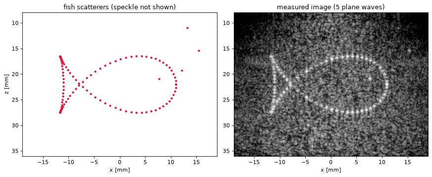
The measured image looks like a routine clinical B-mode: speckle from the diffuse scatterers, the fish outline standing ~25 dB above it, and a receiver-noise floor. This image is the only input the inversions below see — recovering the channel data behind a speckle-and-noise image is considerably harder than in a sterile point-target scene.

Direct inversion: the pseudo-inverse

`invert_direct <../../_autosummary/zea.inverse.rst>`__ treats every sample of the channel-data cube as a free variable and minimizes ||beamform(channel_data) - image||^2 with CGLS. Started from zero, CGLS converges to the minimum-norm least-squares solution — the Moore–Penrose pseudo-inverse applied to the image.

result_direct = invert_direct(operator, image_measured, n_iter=n_iter_direct, verbose=True)


def correlation(a, b):
    """Absolute normalized correlation between two arrays."""
    a = np.asarray(ops.convert_to_numpy(a)).ravel()
    b = np.asarray(ops.convert_to_numpy(b)).ravel()
    a, b = a - a.mean(), b - b.mean()
    return abs(np.vdot(a, b)) / (np.linalg.norm(a) * np.linalg.norm(b) + 1e-30)


print(
    "pre-BF (channel data) correlation: "
    f"{correlation(result_direct.channel_data, channel_data_true):.3f}"
)
print(f"post-BF (image) correlation:       {correlation(result_direct.image, image_measured):.3f}")

zea: cgls iteration   3 | relative residual 5.6788e-01
zea: cgls iteration   6 | relative residual 3.4104e-01
zea: cgls iteration   9 | relative residual 2.0919e-01
zea: cgls iteration  12 | relative residual 1.4435e-01
zea: cgls iteration  15 | relative residual 1.0129e-01
zea: cgls iteration  18 | relative residual 7.5587e-02
zea: cgls iteration  21 | relative residual 6.2533e-02
zea: cgls iteration  24 | relative residual 5.1358e-02
zea: cgls iteration  27 | relative residual 4.4326e-02
zea: cgls iteration  30 | relative residual 3.8029e-02
pre-BF (channel data) correlation: 0.560
post-BF (image) correlation:       0.999

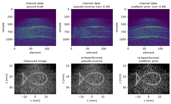
The image fit is essentially perfect while the channel-data correlation is poor — the minimum-norm solution concentrates energy where the beamformer samples, not where the physical echoes are. This is the nullspace problem in action.

Scatterer-prior inversion

`invert_scatterers <../../_autosummary/zea.inverse.rst>`__ instead represents the medium as point scatterers: positions are seeded from the image envelope (`seed_scatterers <../../_autosummary/zea.inverse.rst>`__), and their magnitudes are solved with CGLS through the composition beamform(simulate(positions, magnitudes)) — still a linear problem, but now constrained to physically consistent echoes.

result_scat = invert_scatterers(
    operator,
    image_measured,
    n_scatterers=n_scatterers,
    n_iter=n_iter_scatterers,
    seed=0,
    verbose=True,
)
print(
    "pre-BF (channel data) correlation: "
    f"{correlation(result_scat.channel_data, channel_data_true):.3f}"
)
print(f"post-BF (image) correlation:       {correlation(result_scat.image, image_measured):.3f}")

zea: cgls iteration   7 | relative residual 5.3093e-01
zea: cgls iteration  14 | relative residual 4.5342e-01
zea: cgls iteration  21 | relative residual 4.2392e-01
zea: cgls iteration  28 | relative residual 4.0722e-01
zea: cgls iteration  35 | relative residual 3.9811e-01
zea: cgls iteration  42 | relative residual 3.9201e-01
zea: cgls iteration  49 | relative residual 3.8753e-01
zea: cgls iteration  56 | relative residual 3.8430e-01
zea: cgls iteration  60 | relative residual 3.8237e-01
pre-BF (channel data) correlation: 0.658
post-BF (image) correlation:       0.924

Comparing the recovered channel data

The channel data is the quantity that is never directly observed — below we compare it (for the center transmit) between ground truth and the two inversions, together with the re-beamformed images.

tx = 1  # center (zero-angle) transmit
panels = [
    (channel_data_true, "ground truth"),
    (result_direct.channel_data, "pseudo-inverse"),
    (result_scat.channel_data, "scatterer prior"),
]

fig, axes = plt.subplots(2, 3, figsize=(9, 5.5))
for ax, (cube, title) in zip(axes[0], panels):
    cube = np.asarray(ops.convert_to_numpy(cube))
    label = "" if title == "ground truth" else f" (corr {correlation(cube, channel_data_true):.2f})"
    ax.imshow(
        np.abs(cube[tx]), aspect="auto", cmap="viridis", vmax=np.percentile(np.abs(cube[tx]), 99.5)
    )
    ax.set_title(f"channel data:\n{title}{label}", fontsize=10)
    ax.set(xlabel="element", ylabel="sample")

images = [(image_measured, "measured image")] + [
    (result.image, f"re-beamformed:\n{title}")
    for result, (_, title) in zip([result_direct, result_scat], panels[1:])
]
for ax, (flat, title) in zip(axes[1], images):
    ax.imshow(to_bmode(flat), cmap="gray", vmin=-50, vmax=0, extent=extent, aspect="equal")
    ax.set_title(title, fontsize=10)
    ax.set(xlabel="x [mm]", ylabel="z [mm]")
plt.tight_layout()
plt.show()

Takeaways

• The acquisition is realistic — an L11-5v probe, bandwidth-shaped two-way pulse, tissue speckle and receiver noise — and both inversions still fit the image well — the post-beamformed image barely constrains which channel data produced it.

• The scatterer prior recovers more of the physical channel data (the hyperbolic echo signatures in the top row): its parameterization regularizes the ~n_el * n_tx-fold nullspace of the DAS operator.

• The bright fish points are recovered well; the diffuse speckle floor is much harder — a real physical limitation. The next tutorials show the same gap on recorded data: the CIRS point phantom (0.84) vs the in-vivo carotid (0.06).

• Everything here is backend-agnostic Keras: the same code runs on JAX, TensorFlow and PyTorch. See the `zea.inverse API reference <../../_autosummary/zea.inverse.rst>`__ for the full documentation, including joint position refinement (refine_iters) with `zea.backend.optimizer.adam <../../_autosummary/zea.backend.optimizer.rst>`__.