Inverse beamforming on an in-vivo carotid scan
This tutorial applies `zea.inverse <../../_autosummary/zea.inverse.rst>`__ to an in-vivo carotid acquisition (149 single-element transmits, 128 elements, from the off-grid-ultrasound dataset of van de Schaft et al., arXiv:2407.02285) and reproduces the in-vivo result of the standalone DAS-inversion study: a scatterer-prior inversion with 30,000 scatterers,
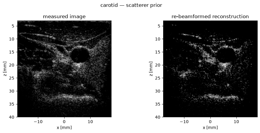
reference pre-BF corr 0.06 and post-BF corr 0.95 (the study ran 70 CGLS iterations; we stop at 40, which captures nearly all of the attainable correlation).
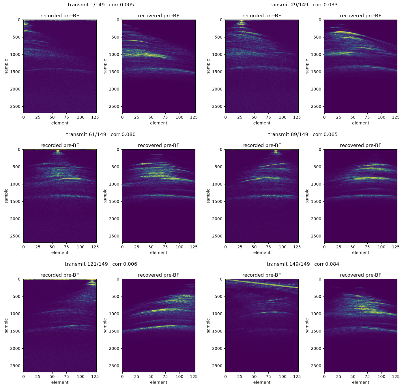
That pre-BF correlation of ≈0.06 is the honest headline: a compounded image constrains speckle statistics, not the specific channel-data realization, so recovering diffuse in-vivo channel data from one image is fundamentally limited. Compare the CIRS phantom tutorial (0.84 on point targets) and the introductory tutorial, which sits between the two regimes with bright points over speckle.


‼️ Important: This notebook is optimized for GPU/TPU. Code execution on a CPU may be very slow.
If you are running in Colab, please enable a hardware accelerator via:
Runtime → Change runtime type → Hardware accelerator → GPU/TPU 🚀.
[1]:
%%capture
%pip install zea
[2]:
import os

os.environ["KERAS_BACKEND"] = "jax"
os.environ["TF_CPP_MIN_LOG_LEVEL"] = "3"

import time
import urllib.request
from pathlib import Path

import h5py
import matplotlib.pyplot as plt
import numpy as np
from keras import ops
from matplotlib.animation import FuncAnimation, PillowWriter

import zea
from zea.inverse import DASOperator, ScattererSimulator, invert_scatterers

zea.init_device()
zea: Using backend 'jax'
-------------------GPU settings-------------------
0/1 GPUs were disabled
     memory
GPU
0       81072
Selecting 1 GPU based on available memory.
Selected GPU 0 with Free Memory: 81072.00 MiB
--------------------------------------------------
[2]:
'gpu:0'
[3]:
# Parameters (overridden for fast CI runs, see tests/test_notebooks.py)
# CGLS is stopped early: on ill-posed problems the iteration count doubles as
# the regularization parameter, and 40 iterations capture nearly all of the
# attainable correlation at a fraction of the runtime.
n_iter = 40
n_scatterers = 30000
# The scan is a 411 MB download and the inversion runs for hours; CI skips it.
run_inversion = True
Download the scan
The in-vivo carotid scan (411 MB) comes from the off-grid-ultrasound dataset on Zenodo. It is in the (legacy) zea HDF5 format and loads directly with `zea.File <../../_autosummary/zea.data.file.rst>`__. We use this specific scan so the results are directly comparable with the original study; for more zea-native carotid data see the `zeahub/zea-carotid-2023 <https://huggingface.co/datasets/zeahub/zea-carotid-2023>`__ dataset, which zea.File opens straight from hf:// URLs.
[4]:
DATA_DIR = Path(os.environ.get("ZEA_INVERSE_DATA_DIR", "~/zea-inverse-data")).expanduser()
DATA_DIR.mkdir(parents=True, exist_ok=True)

SCAN_PATH = DATA_DIR / "L11-5v_carotid1.hdf5"
SCAN_URL = "https://zenodo.org/records/14925758/files/L11-5v_carotid1.hdf5?download=1"

if run_inversion and not SCAN_PATH.exists():
    print(f"downloading {SCAN_PATH.name} (411 MB) ...")
    urllib.request.urlretrieve(SCAN_URL, SCAN_PATH)
    print(f"  -> {SCAN_PATH} ({SCAN_PATH.stat().st_size / 1e6:.0f} MB)")
Loading a scan for inversion
We load the acquisition into `zea.Parameters <../../parameters_doc.rst>`__ with a few overrides that match the conventions of the original study:
``t_peak``: the original beamformer used the two-way waveform’s time-to-peak, doubled (a jaxus convention). We override
t_peakaccordingly so the delay model matches exactly.``element_width``: these legacy files store the element width under
scan/, which the legacy loader drops — we read it directly and pass it as an override (it drives the element directivity model in the simulator).grid: a 0.6-wavelength pixel grid over the imaging region, and a receive f-number of 1.5 (the original configuration).
[5]:
def load_scan(path, region, pixels_per_wavelength=1 / 0.6, f_number=1.5, frame=0):
    """Load a scan and its raw RF data with the original study's conventions."""
    with h5py.File(path, "r") as h:
        element_width = float(h["scan/element_width"][()])
    with zea.File(path) as file:
        parameters = file.load_parameters()
        raw_data = np.asarray(file["data/raw_data"][frame, ..., 0], dtype=np.float32)

    # t_peak: two-way waveform peak time, doubled (jaxus/original-study convention)
    waveform = np.asarray(parameters.waveforms_two_way[0])
    t_peak = np.full(parameters.n_tx, 2.0 * np.argmax(waveform) / 250e6, dtype=np.float32)

    # 0.6-wavelength pixel grid over the requested region
    spacing = parameters.sound_speed / float(np.mean(parameters.center_frequency))
    spacing = spacing / pixels_per_wavelength
    grid_size_x = int((region[1] - region[0]) / spacing) + 1
    grid_size_z = int((region[3] - region[2]) / spacing) + 1

    with zea.File(path) as file:
        parameters = file.load_parameters(
            t_peak=t_peak,
            element_width=element_width,
            f_number=f_number,
            xlims=(region[0], region[1]),
            zlims=(region[2], region[3]),
            grid_size_x=grid_size_x,
            grid_size_z=grid_size_z,
        )
    print(
        f"{Path(path).name}: n_tx={parameters.n_tx} n_el={parameters.n_el} "
        f"n_ax={parameters.n_ax} grid=({grid_size_z}, {grid_size_x})"
    )
    return parameters, raw_data


def correlation(a, b):
    """Absolute normalized correlation between two arrays."""
    a = np.asarray(ops.convert_to_numpy(a)).ravel()
    b = np.asarray(ops.convert_to_numpy(b)).ravel()
    a, b = a - a.mean(), b - b.mean()
    return abs(np.vdot(a, b)) / (np.linalg.norm(a) * np.linalg.norm(b) + 1e-30)


def report(label, result, raw_data, image, reference):
    """Print pre/post-beamforming correlations next to the reference values."""
    pre = correlation(result.channel_data, raw_data)
    post = correlation(result.image, image)
    print(
        f"{label:28s} pre-BF corr {pre:.3f} (reference {reference[0]:.3f})   "
        f"post-BF corr {post:.3f} (reference {reference[1]:.3f})"
    )
    return pre, post
Rendering helpers
show_images compares the measured image with the re-beamformed reconstruction (log-compressed |RF|, as in the original study). render_prebf_gif animates the recovered pre-beamformed channel data across transmits next to the recorded ground truth — this is the quantity being recovered, which the inversion never observes.
[6]:
def to_db(image_2d):
    magnitude = np.abs(image_2d)
    return 20 * np.log10(magnitude / (magnitude.max() + 1e-12) + 1e-6)


def show_images(operator, image, result, region, scatterers=None, title=""):
    extent = [region[0] * 1e3, region[1] * 1e3, region[3] * 1e3, region[2] * 1e3]
    fig, axes = plt.subplots(1, 2, figsize=(10, 4.5))
    panels = [(image, "measured image"), (result.image, "re-beamformed reconstruction")]
    for ax, (flat, label) in zip(axes, panels):
        ax.imshow(
            to_db(ops.convert_to_numpy(operator.to_grid(flat))),
            cmap="gray",
            vmin=-50,
            vmax=0,
            extent=extent,
            aspect="equal",
        )
        if scatterers is not None:
            ax.scatter(
                scatterers[:, 0] * 1e3,
                scatterers[:, 2] * 1e3,
                s=16,
                facecolors="none",
                edgecolors="r",
                linewidths=0.8,
            )
        ax.set(title=label, xlabel="x [mm]", ylabel="z [mm]")
    fig.suptitle(title)
    plt.tight_layout()
    plt.show()


def render_prebf_gif(filename, channel_data_true, channel_data_recon, transmits, fps=10):
    """Animate ground-truth vs recovered channel data across transmits."""
    gt = np.asarray(ops.convert_to_numpy(channel_data_true))
    recon = np.asarray(ops.convert_to_numpy(channel_data_recon))
    fig, axes = plt.subplots(1, 2, figsize=(7, 4.5))

    def draw(tx):
        for ax in axes:
            ax.clear()
        for ax, cube, label in zip(axes, [gt, recon], ["recorded pre-BF", "recovered pre-BF"]):
            ax.imshow(
                np.abs(cube[tx]),
                aspect="auto",
                cmap="viridis",
                vmax=np.percentile(np.abs(cube[tx]), 99.5) + 1e-12,
            )
            ax.set(title=label, xlabel="element", ylabel="sample")
        tx_corr = correlation(recon[tx], gt[tx])
        fig.suptitle(f"transmit {tx + 1}/{gt.shape[0]}   corr {tx_corr:.3f}")
        fig.tight_layout()

    animation = FuncAnimation(fig, draw, frames=list(transmits), interval=1000 / fps)
    animation.save(filename, writer=PillowWriter(fps=fps))
    plt.close(fig)
    print(f"saved {filename} ({Path(filename).stat().st_size / 1e6:.1f} MB)")
Scatterer-prior inversion
We beamform the recorded channel data once to get the measured image — from here on, the inversion sees only that image. 30,000 scatterers are seeded from the image envelope and their magnitudes solved with CGLS.
[7]:
REGION_CAROTID = (-0.018, 0.018, 0.003, 0.04)

if run_inversion:
    parameters, raw_data = load_scan(SCAN_PATH, REGION_CAROTID)
    operator = DASOperator(parameters)
    image = operator.forward(raw_data)

    start = time.time()
    simulator = ScattererSimulator(parameters, chunk_size=4096)
    result_carotid = invert_scatterers(
        operator,
        image,
        n_scatterers=n_scatterers,
        n_iter=n_iter,
        seed=0,
        simulator=simulator,
    )
    print(f"scatterer-prior inversion: {time.time() - start:.0f}s")
    report("carotid scatterer prior (30k)", result_carotid, raw_data, image, (0.057, 0.946))
zea: WARNING This ``zea.File`` '/nfs/scistore20/bronsgrp/svedula/das-inversion/data/L11-5v_carotid1.hdf5' was created with a legacy version of zea (<0.1.0), while you are using zea v0.1.2. It may behave in unexpected ways. Install an earlier version of zea<0.1.0 for full compatibility or re-save the file with zea v0.1.0 or later (e.g. via File.create).
zea: WARNING The waveforms_one_way parameter is stored as a dictionary in the file. Converting to array. This will be deprecated in future versions of zea. Please update your files to store waveforms as arrays of shape `(n_tx, n_samples)`.
zea: WARNING The waveforms_two_way parameter is stored as a dictionary in the file. Converting to array. This will be deprecated in future versions of zea. Please update your files to store waveforms as arrays of shape `(n_tx, n_samples)`.
zea: WARNING The waveforms_one_way parameter is stored as a dictionary in the file. Converting to array. This will be deprecated in future versions of zea. Please update your files to store waveforms as arrays of shape `(n_tx, n_samples)`.
zea: WARNING The waveforms_two_way parameter is stored as a dictionary in the file. Converting to array. This will be deprecated in future versions of zea. Please update your files to store waveforms as arrays of shape `(n_tx, n_samples)`.
L11-5v_carotid1.hdf5: n_tx=149 n_el=128 n_ax=2688 grid=(305, 297)
zea: WARNING width/grid_size_x = 0.0001212 > wavelength/2 = 0.0001013. Consider increasing grid_size_x to 356 or more, or unsetting it to size the grid automatically.
zea: WARNING depth/grid_size_z = 0.0001213 > wavelength/2 = 0.0001013. Consider increasing grid_size_z to 366 or more, or unsetting it to size the grid automatically.
scatterer-prior inversion: 1307s
carotid scatterer prior (30k) pre-BF corr 0.060 (reference 0.057)   post-BF corr 0.931 (reference 0.946)
[8]:
if run_inversion:
    show_images(operator, image, result_carotid, REGION_CAROTID, title="carotid — scatterer prior")
    render_prebf_gif(
        "carotid_prebf.gif",
        raw_data,
        result_carotid.channel_data,
        transmits=range(0, parameters.n_tx, 4),  # subsample transmits to keep the GIF small
        fps=10,
    )
saved carotid_prebf.gif (4.1 MB)
Takeaways
The inversion reproduces the reference result of the original study.
The re-beamformed image matches the measured image well (post-BF corr ≈0.95), yet the channel data itself stays unrecoverable (pre-BF corr ≈0.06): in-vivo speckle lives almost entirely in the nullspace of the compounded DAS operator.
This ceiling is fundamental, not a tuning issue — the image simply does not carry the channel-data micro-realization. Bright point targets are a different story: see the CIRS phantom tutorial.